Fourth-Order Runge-Kutta Method to Solve Differential Equations

Introduction

A calculator to solve differential equations of the second order using a numerical method based on the Fourth Order Runge-Kutta Method [1] and a calculator-based analytical method is presented for comparison and educational purposes.
The fourth-order Runge-Kutta method applied to a first-order differential equation is presented and then the same method is applied to a second order linear differential equation. Finally, an interactive tutorial to study the effects of the step size \( h \) used in the Runga-Kutta method is included.

Fourth-Order Runge-Kutta Method to a First-Order Differential Equation

The 4th Order Runge-Kutta method is a numerical method widely used to solve ordinary differential equations (ODEs) of the form: \[ \dfrac{dy}{dt} = f(y, t) \] with an initial condition \( y(0) = y_0 \). The 4th Order Runge-Kutta method approximates the solution \( y(t) \) at a future time \( t + h \) (where \( h \) is the step size) based on the information at time \( t \). The method uses four intermediate steps to compute the slope at different points within the interval \([t, t+h]\) and combines them to get a weighted average slope, which is then used to estimate \( y(t+h) \). Here are the steps involved in the 4th Order Runge-Kutta method:
Step 1: \[ k_1 = h \cdot f(y_n, t_n) \] Here, \( y_n \) and \( t_n \) are the current values of \( y \) and \( t \).
Step 2: \[ k_2 = h \cdot f\left(y_n + \dfrac{k_1}{2}, t_n + \dfrac{h}{2}\right) \] Step 3: \[ k_3 = h \cdot f\left(y_n + \dfrac{k_2}{2}, t_n + \dfrac{h}{2}\right) \] Step 4: \[ k_4 = h \cdot f(y_n + k_3, t_n + h) \] Step 5:
Update \( y \) and \( t \) The fourth-order Runge-Kutta method combines the above quantities (slopes) to approximate the value of \( y \) at the end of the interval \([t, t+h]\). The weighted average of these slopes is calculated using the formula: \[ \dfrac{1}{6}(k_1 + 2k_2 + 2k_3 + k_4) \] This average slope is then multiplied by \( h \) and added to \( y_n \) to update the value of \( y \) at \( t_{n+1} \). \[ y_{n+1} = y_n + h (\dfrac{1}{6}(k_1 + 2k_2 + 2k_3 + k_4)) \] \[ t_{n+1} = t_n + h \]

Runge-Kutta Method to a Second-Order Differential Equation

For a second-order differential equation of the form: \[ \dfrac{d^2y}{dt^2} = f(y, \dfrac{dy}{dt}, t) \] with initial conditions: \[ y(0) = y_0 \] \[ \dfrac{dy}{dt}(0) = \dfrac{dy}{dt}_0 \] we can convert it into a system of two first-order differential equations by introducing a new variable:
Let \[ \dfrac{dy}{dt} = v \] Thus, the second order differential equation may be written as system as follows: \[ \dfrac{dy}{dt} = v \] \[ \dfrac{dv}{dt} = \dfrac{d^2y}{dt^2} = f(y, v, t) \] We can then use the 4th Order Runge-Kutta method to solve this system of first-order differential equations as follows:
Step 1:
Compute \( k_{1y} \) and \( k_{1v} \) \[ k_{1y} = h \cdot v \] \[ k_{1v} = h \cdot f(y_n, v_n, t_n) \]
Step 2:
Compute \( k_{2y} \) and \( k_{2v} \) \[ k_{2y} = h \cdot (v_n + \dfrac{k_{1v}}{2}) \] \[ k_{2v} = h \cdot f\left(y_n + \dfrac{k_{1y}}{2}, v_n + \dfrac{k_{1v}}{2}, t_n + \dfrac{h}{2}\right) \]
Step 3:
Compute \( k_{3y} \) and \( k_{3v} \) \[ k_{3y} = h \cdot (v_n + \dfrac{k_{2v}}{2}) \] \[ k_{3v} = h \cdot f\left(y_n + \dfrac{k_{2y}}{2}, v_n + \dfrac{k_{2v}}{2}, t_n + \dfrac{h}{2}\right) \]
Step 4:
Compute \( k_{4y} \) and \( k_{4v} \) \[ k_{4y} = h \cdot (v_n + k_{3v}) \] \[ k_{4v} = h \cdot f(y_n + k_{3y}, v_n + k_{3v}, t_n + h) \]
Step 5:
Update \( y \) and \( v \) \[ y_{n+1} = y_n + \dfrac{1}{6}(k_{1y} + 2k_{2y} + 2k_{3y} + k_{4y}) \] \[ v_{n+1} = v_n + \dfrac{1}{6}(k_{1v} + 2k_{2v} + 2k_{3v} + k_{4v}) \] \[ t_{n+1} = t_n + h \]

Runge-Kutta Method Calculator

We now present a calculator that approximates the solution to the second-order differential equations of the form \[ a \dfrac{d^2y}{dt^2} + b \dfrac{dy}{dt} + c y = 0 \] using the fourth-order Runge-Kutta method described above and the solution is also given analytically for comparison.
The above differential equation is also solved analytically to make comparisons.
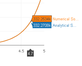
Let \[ \dfrac{dy}{dt} = v \] We therefore need to apply the 4th Order Runge-Kutta method to the following system. \[ \dfrac{dy}{dt} = v \] \[ \dfrac{dv}{dt} = \dfrac{d^2y}{dt^2} = \dfrac{1}{a} (- b \; v - c \; y ) \] The calculator uses the fourth order Runge-Kutta method and also solves the same differential equation analytically and compare the results graphically.

Enter Coefficients and Initial Conditions

Enter the coefficients \(a, b \) and \( c \) as well as the initial conditions \( y(0) \) and \( dy/dt(0) \) and the step size \( h \), then solve and compare the graphs of the numerical and analytical solutions obtained.
Note
1) You may use the mousse and hover above the graphs to obtain a reading of points on the graphs and therefore compare them.
Reading points on a graph
2) Use the mousse to display one graph at a time or both by clicking on the graphs in the legend shown on the right side.
Graph legend
3) The errors in using the Runge-Kutta method depend on the step size \( h \). This calculator allows to change \( h \) and therefore compares the numerical and the analytical methods and studies the effect of \( h \) on the errors due to the approximation used in the 4th Order Runge-Kutta method.
4) You may also change the number \( n \) of steps used in the calculations. The graph extends from \( x = 0 \) to \( x = n \times h \).

a:
b:
c:
y(0):
dy/dt(0):
Step size: \( h \)
Number of Steps: \( n \)

Solutions:

Interactive Tutorial: Effects of the Size of the step \( h \) on the Approximation by Ruga-Kutta Method

Enter the following values for the constants \( b , c \) and \( d \) as follows:
\( a = 1 \) , \( b = 0.5 \) and \( c = 5 \) which should give an oscilating function with decreasing amplitude.
Now enter values of \( h \) starting from \( h = 0.01 \) and then increase \( h \) up to 1. Which values of \( h \) give a better approximation to the solution when compared to the analytical method?